scikit-opt

Python

Python实现的群体智能算法（遗传算法、粒子群优化、模拟退火、蚁群算法、免疫算法、人工鱼群算法的Python实现）

文档: https://scikit-opt.github.io/scikit-opt/#/en/
文档： https://scikit-opt.github.io/scikit-opt/#/zh/
源代码: https://github.com/guofei9987/scikit-opt
帮助我们改进scikit-opt https://www.wjx.cn/jq/50964691.aspx

安装

pip install scikit-opt

对于当前开发版本：

git clone git@github.com:guofei9987/scikit-opt.git
cd scikit-opt
pip install .

特性

特性1：UDF

现在支持UDF（用户自定义函数）！

例如，你刚刚开发了一种新的选择函数。现在，你的选择函数如下所示： -> 示例代码：examples/demo_ga_udf.py#s1

# 步骤1：定义你自己的操作符：
def selection_tournament(algorithm, tourn_size):
    FitV = algorithm.FitV
    sel_index = []
    for i in range(algorithm.size_pop):
        aspirants_index = np.random.choice(range(algorithm.size_pop), size=tourn_size)
        sel_index.append(max(aspirants_index, key=lambda i: FitV[i]))
    algorithm.Chrom = algorithm.Chrom[sel_index, :]  # 下一代
    return algorithm.Chrom

导入并构建遗传算法 -> 示例代码：examples/demo_ga_udf.py#s2

import numpy as np
from sko.GA import GA, GA_TSP

demo_func = lambda x: x[0] ** 2 + (x[1] - 0.05) ** 2 + (x[2] - 0.5) ** 2
ga = GA(func=demo_func, n_dim=3, size_pop=100, max_iter=500, prob_mut=0.001,
        lb=[-1, -10, -5], ub=[2, 10, 2], precision=[1e-7, 1e-7, 1])

将你的自定义函数注册到遗传算法中 -> 示例代码：examples/demo_ga_udf.py#s3

ga.register(operator_name='selection', operator=selection_tournament, tourn_size=3)

scikit-opt还提供了一些操作符 -> 示例代码：examples/demo_ga_udf.py#s4

from sko.operators import ranking, selection, crossover, mutation

ga.register(operator_name='ranking', operator=ranking.ranking). \
    register(operator_name='crossover', operator=crossover.crossover_2point). \
    register(operator_name='mutation', operator=mutation.mutation)

现在像往常一样运行遗传算法 -> 示例代码：examples/demo_ga_udf.py#s5

best_x, best_y = ga.run()
print('best_x:', best_x, '\n', 'best_y:', best_y)

目前，udf支持遗传算法的交叉、变异、选择和排序 scikit-opt提供了十几种操作符，详见这里

对于高级用户：

-> 示例代码：examples/demo_ga_udf.py#s6

class MyGA(GA):
    def selection(self, tourn_size=3):
        FitV = self.FitV
        sel_index = []
        for i in range(self.size_pop):
            aspirants_index = np.random.choice(range(self.size_pop), size=tourn_size)
            sel_index.append(max(aspirants_index, key=lambda i: FitV[i]))
        self.Chrom = self.Chrom[sel_index, :]  # 下一代
        return self.Chrom

    ranking = ranking.ranking


demo_func = lambda x: x[0] ** 2 + (x[1] - 0.05) ** 2 + (x[2] - 0.5) ** 2
my_ga = MyGA(func=demo_func, n_dim=3, size_pop=100, max_iter=500, lb=[-1, -10, -5], ub=[2, 10, 2],
             precision=[1e-7, 1e-7, 1])
best_x, best_y = my_ga.run()
print('best_x:', best_x, '\n', 'best_y:', best_y)

特性2：继续运行

（0.3.6版本新增）运行算法10次迭代，然后基于前10次迭代再运行20次迭代：

from sko.GA import GA

func = lambda x: x[0] ** 2
ga = GA(func=func, n_dim=1)
ga.run(10)
ga.run(20)

特性3：4种加速方式

向量化
多线程
多进程
缓存

详见 https://github.com/guofei9987/scikit-opt/blob/master/examples/example_function_modes.py

特性4：GPU计算

我们正在开发GPU计算功能，将在1.0.0版本稳定发布。目前已有可用示例：https://github.com/guofei9987/scikit-opt/blob/master/examples/demo_ga_gpu.py

快速入门

1. 差分进化算法

第1步：定义问题
-> 示例代码：examples/demo_de.py#s1

'''
最小化 f(x1, x2, x3) = x1^2 + x2^2 + x3^2
约束条件：
    x1*x2 >= 1
    x1*x2 <= 5
    x2 + x3 = 1
    0 <= x1, x2, x3 <= 5
'''

def obj_func(p):
    x1, x2, x3 = p
    return x1 ** 2 + x2 ** 2 + x3 ** 2

constraint_eq = [
    lambda x: 1 - x[1] - x[2]
]

constraint_ueq = [
    lambda x: 1 - x[0] * x[1],
    lambda x: x[0] * x[1] - 5
]

第2步：执行差分进化算法
-> 示例代码：examples/demo_de.py#s2

from sko.DE import DE

de = DE(func=obj_func, n_dim=3, size_pop=50, max_iter=800, lb=[0, 0, 0], ub=[5, 5, 5],
        constraint_eq=constraint_eq, constraint_ueq=constraint_ueq)

best_x, best_y = de.run()
print('最优解:', best_x, '\n', '最优值:', best_y)

2. 遗传算法

第1步：定义问题
-> 示例代码：examples/demo_ga.py#s1

import numpy as np

def schaffer(p):
    '''
    该函数有大量局部最小值，具有强烈震荡
    全局最小值在(0,0)处，取值为0
    https://en.wikipedia.org/wiki/Test_functions_for_optimization
    '''
    x1, x2 = p
    part1 = np.square(x1) - np.square(x2)
    part2 = np.square(x1) + np.square(x2)
    return 0.5 + (np.square(np.sin(part1)) - 0.5) / np.square(1 + 0.001 * part2)

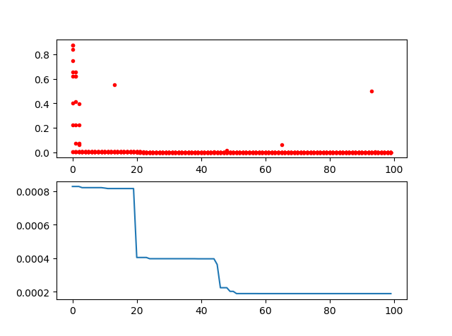
第2步：执行遗传算法
-> 示例代码：examples/demo_ga.py#s2

from sko.GA import GA

ga = GA(func=schaffer, n_dim=2, size_pop=50, max_iter=800, prob_mut=0.001, lb=[-1, -1], ub=[1, 1], precision=1e-7)
best_x, best_y = ga.run()
print('最优解:', best_x, '\n', '最优值:', best_y)

-> 示例代码：examples/demo_ga.py#s3

import pandas as pd
import matplotlib.pyplot as plt

Y_history = pd.DataFrame(ga.all_history_Y)
fig, ax = plt.subplots(2, 1)
ax[0].plot(Y_history.index, Y_history.values, '.', color='red')
Y_history.min(axis=1).cummin().plot(kind='line')
plt.show()

Figure_1-1

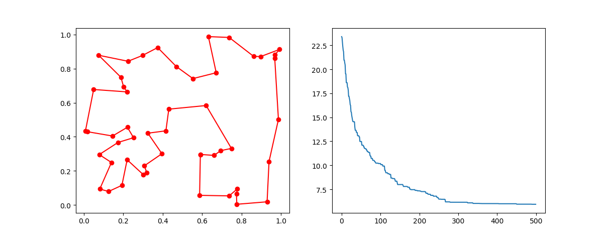
2.2 用于TSP（旅行商问题）的遗传算法

只需导入GA_TSP，它重载了crossover和mutation以解决TSP问题

第1步：定义问题。准备好点的坐标和距离矩阵。
这里我随机生成数据作为演示：
-> 示例代码：examples/demo_ga_tsp.py#s1

import numpy as np
from scipy import spatial
import matplotlib.pyplot as plt

num_points = 50

points_coordinate = np.random.rand(num_points, 2)  # 生成点的坐标
distance_matrix = spatial.distance.cdist(points_coordinate, points_coordinate, metric='euclidean')

def cal_total_distance(routine):
    '''目标函数。输入路线，返回总距离。
    cal_total_distance(np.arange(num_points))
    '''
    num_points, = routine.shape
    return sum([distance_matrix[routine[i % num_points], routine[(i + 1) % num_points]] for i in range(num_points)])

第2步：执行遗传算法
-> 示例代码：examples/demo_ga_tsp.py#s2

from sko.GA import GA_TSP

ga_tsp = GA_TSP(func=cal_total_distance, n_dim=num_points, size_pop=50, max_iter=500, prob_mut=1)
best_points, best_distance = ga_tsp.run()

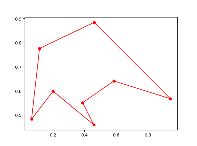
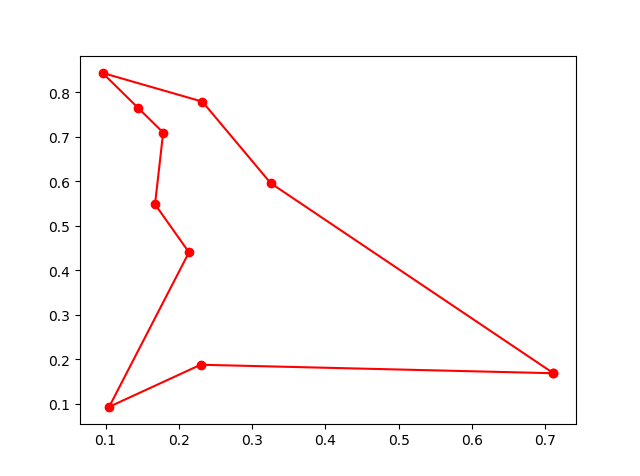
第3步：绘制结果：
-> 示例代码：examples/demo_ga_tsp.py#s3

fig, ax = plt.subplots(1, 2)
best_points_ = np.concatenate([best_points, [best_points[0]]])
best_points_coordinate = points_coordinate[best_points_, :]
ax[0].plot(best_points_coordinate[:, 0], best_points_coordinate[:, 1], 'o-r')
ax[1].plot(ga_tsp.generation_best_Y)
plt.show()

GA_TPS

3. PSO（粒子群优化）

3.1 粒子群优化算法（PSO）

步骤1：定义你的问题： -> 示例代码：examples/demo_pso.py#s1

def demo_func(x):
    x1, x2, x3 = x
    return x1 ** 2 + (x2 - 0.05) ** 2 + x3 ** 2

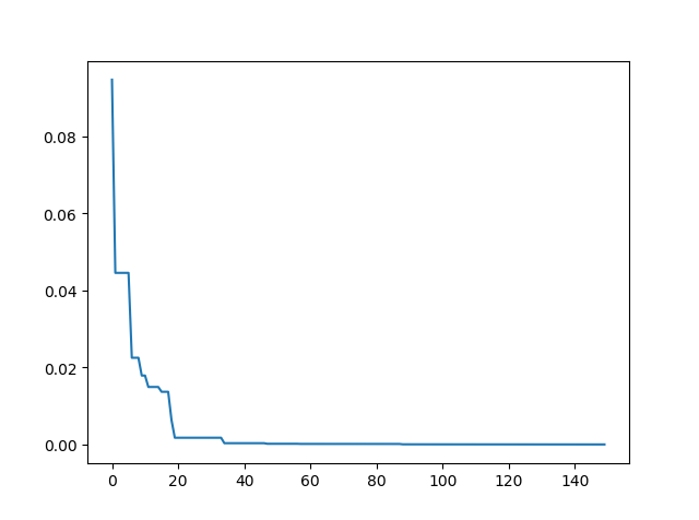
步骤2：执行PSO -> 示例代码：examples/demo_pso.py#s2

from sko.PSO import PSO

pso = PSO(func=demo_func, n_dim=3, pop=40, max_iter=150, lb=[0, -1, 0.5], ub=[1, 1, 1], w=0.8, c1=0.5, c2=0.5)
pso.run()
print('最优x为', pso.gbest_x, '最优y为', pso.gbest_y)

步骤3：绘制结果 -> 示例代码：examples/demo_pso.py#s3

import matplotlib.pyplot as plt

plt.plot(pso.gbest_y_hist)
plt.show()

PSO_TPS

3.2 带非线性约束的PSO

如果你需要非线性约束，比如 (x[0] - 1) ** 2 + (x[1] - 0) ** 2 - 0.5 ** 2<=0 代码如下：

constraint_ueq = (
    lambda x: (x[0] - 1) ** 2 + (x[1] - 0) ** 2 - 0.5 ** 2
    ,
)
pso = PSO(func=demo_func, n_dim=2, pop=40, max_iter=max_iter, lb=[-2, -2], ub=[2, 2]
          , constraint_ueq=constraint_ueq)

注意，你可以添加多个非线性约束。只需将它们添加到 constraint_ueq 中

此外，我们还有一个动画： pso_ani ↑查看 examples/demo_pso_ani.py

4. 模拟退火算法（SA）

4.1 用于多元函数的SA

步骤1：定义你的问题 -> 示例代码：examples/demo_sa.py#s1

demo_func = lambda x: x[0] ** 2 + (x[1] - 0.05) ** 2 + x[2] ** 2

步骤2：执行SA -> 示例代码：examples/demo_sa.py#s2

from sko.SA import SA

sa = SA(func=demo_func, x0=[1, 1, 1], T_max=1, T_min=1e-9, L=300, max_stay_counter=150)
best_x, best_y = sa.run()
print('最优x:', best_x, '最优y', best_y)

步骤3：绘制结果 -> 示例代码：examples/demo_sa.py#s3

import matplotlib.pyplot as plt
import pandas as pd

plt.plot(pd.DataFrame(sa.best_y_history).cummin(axis=0))
plt.show()

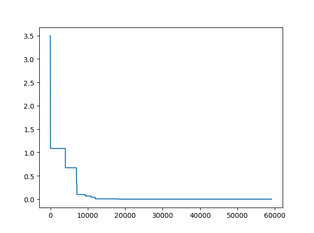
此外，scikit-opt提供了3种类型的模拟退火算法：快速退火、玻尔兹曼退火和柯西退火。查看更多SA信息

4.2 用于TSP的SA

步骤1：哦，是的，定义你的问题。太无聊了，就不复制这一步了。

步骤2：对TSP执行SA -> 示例代码：examples/demo_sa_tsp.py#s2

from sko.SA import SA_TSP

sa_tsp = SA_TSP(func=cal_total_distance, x0=range(num_points), T_max=100, T_min=1, L=10 * num_points)

best_points, best_distance = sa_tsp.run()
print(best_points, best_distance, cal_total_distance(best_points))

步骤3：绘制结果 -> 示例代码：examples/demo_sa_tsp.py#s3

from matplotlib.ticker import FormatStrFormatter

fig, ax = plt.subplots(1, 2)

best_points_ = np.concatenate([best_points, [best_points[0]]])
best_points_coordinate = points_coordinate[best_points_, :]
ax[0].plot(sa_tsp.best_y_history)
ax[0].set_xlabel("迭代次数")
ax[0].set_ylabel("距离")
ax[1].plot(best_points_coordinate[:, 0], best_points_coordinate[:, 1],
           marker='o', markerfacecolor='b', color='c', linestyle='-')
ax[1].xaxis.set_major_formatter(FormatStrFormatter('%.3f'))
ax[1].yaxis.set_major_formatter(FormatStrFormatter('%.3f'))
ax[1].set_xlabel("经度")
ax[1].set_ylabel("纬度")
plt.show()

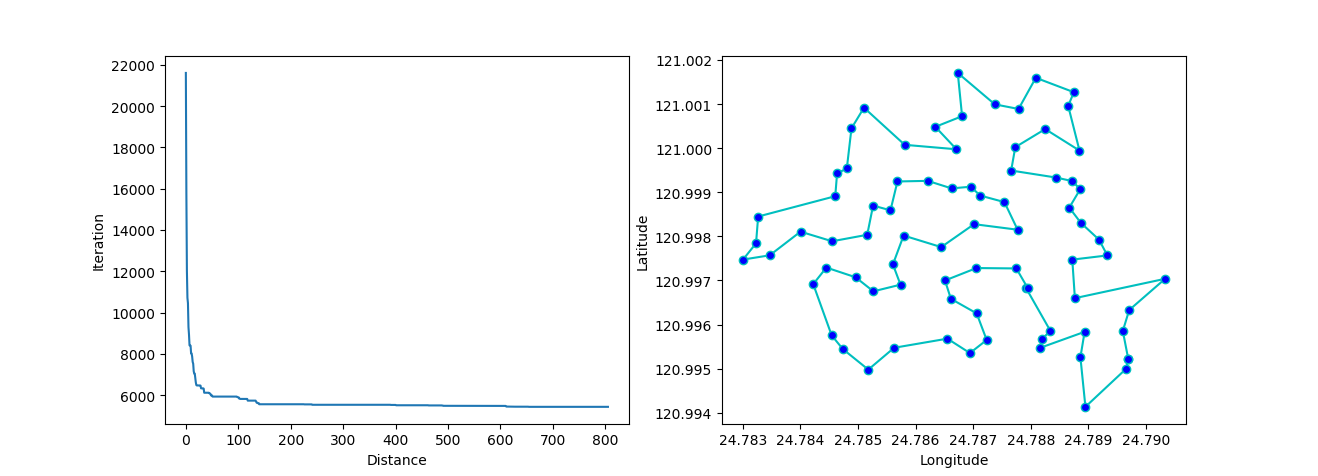
更多：绘制动画：

↑查看 examples/demo_sa_tsp.py

5. 用于TSP的蚁群算法（ACA）

-> 示例代码：examples/demo_aca_tsp.py#s2

from sko.ACA import ACA_TSP

aca = ACA_TSP(func=cal_total_distance, n_dim=num_points,
              size_pop=50, max_iter=200,
              distance_matrix=distance_matrix)

best_x, best_y = aca.run()

ACA

6. 免疫算法（IA）

-> 示例代码：examples/demo_ia.py#s2


from sko.IA import IA_TSP

ia_tsp = IA_TSP(func=cal_total_distance, n_dim=num_points, size_pop=500, max_iter=800, prob_mut=0.2,
                T=0.7, alpha=0.95)
best_points, best_distance = ia_tsp.run()
print('最佳路线:', best_points, '最短距离:', best_distance)

7. 人工鱼群算法（AFSA）

-> 示例代码：examples/demo_afsa.py#s1

def func(x):
    x1, x2 = x
    return 1 / x1 ** 2 + x1 ** 2 + 1 / x2 ** 2 + x2 ** 2


from sko.AFSA import AFSA

afsa = AFSA(func, n_dim=2, size_pop=50, max_iter=300,
            max_try_num=100, step=0.5, visual=0.3,
            q=0.98, delta=0.5)
best_x, best_y = afsa.run()
print(best_x, best_y)